Statistics
Dr. Larry Genalo
02-24-2013
Prepared by: Walter Bennette
Statistics
Statistics- parameters calculated from sample observations (engineers typically deal with samples rather than the total population)
Examples:
- How much fuel should a gas station keep in stock?
- Who might win the next election?
- What players should go on your fantasy sports team?
- …
Statistics
Measure of AVERAGE (Central Tendency)
Mode: The most common value in a sample
Median: “Middle” value in the sample
Mean: Arithmetic average = \( \bar X = \frac{\sum_{i=1}^N X_i}N \)
Variation

Variation
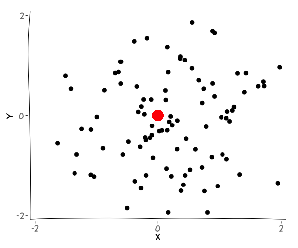
Variation

Variation
Measures of Variation (scatter, dispersal) about the mean:
\[ Variance = S^2 = \frac{\sum_{i = 1}^N ( X_i - \bar X )^2 }{N - 1} \]
\[ Standard \ Deviation = S = \sqrt{S^2} \]
Note: this equation for variance (using N-1) is used for a small sample of a population
Alternative Deviation Equation
An alternative equation to find the standard deviation is the following:
\[ Standard \ Deviation = S = \sqrt{\frac{N \sum (X_i^2) - (\sum X_i)^2}{N(N-1)}} \]
Example
| i | 1 | 2 | 3 | 4 | 5 | 6 |
| \( X_i \) | 92 | 63 | 74 | 63 | 78 | 78 |
- Mode =
- Median =
- Mean =
- Standard Deviation =
- Variance =
It makes these specific calculations easier if the numbers are reordered
Example
| i' | 1 | 2 | 3 | 4 | 5 | 6 |
| \( X_{i'} \) | 63 | 63 | 74 | 78 | 78 | 92 |
\( Mode \) \( = \) \( 63 \) \( and \) \( 78 \)
\( Median = \frac{(78+74)}2 = 76 \)
Example
| i' | 1 | 2 | 3 | 4 | 5 | 6 |
| \( X_{i'} \) | 63 | 63 | 74 | 78 | 78 | 92 |
\( Mean=\bar X = \frac{\sum_{i=1}^N X_i}N \)
\( \bar X = \frac {( 63 + 63 + 74 + 78 +78 +92 )}6 = 74.67 \)
Example
| i' | 1 | 2 | 3 | 4 | 5 | 6 |
| \( X_{i'} \) | 63 | 63 | 74 | 78 | 78 | 92 |
\( Standard \ Deviation = S = \sqrt{\frac{N \sum (X_i^2) - (\sum X_i)^2}{N(N-1)}} \)
\( S = \sqrt{\frac{6 (63^2 + ... + 92^2) - (63 + ... + 92)^2}{6(5)}} = 10.91 \)
Example
| i' | 1 | 2 | 3 | 4 | 5 | 6 |
| \( X_{i'} \) | 63 | 63 | 74 | 78 | 78 | 92 |
\( Variance = S^2 \)
\( S^2 = (10.911767)^2 = 119.1 \)
Example 2
| i | 1 | 2 | 3 | … | 48 |
| \( X_i \) | 85 | 93 | 72 | … | 5 |
| Freq of Occur. |
Grade Class |
|---|---|
| 8 | 90-100 |
| 13 | 80-89 |
| 15 | 70-79 |
| 8 | 60-69 |
| 4 | 0-59 |
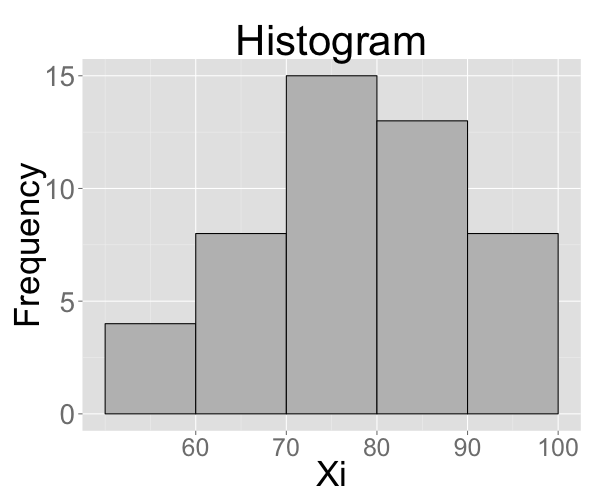
Frequency Distribution
This can lead to a Continuous Distribution such as:

This is an example of a theoretical distribution called the Normal Distribution or a “Bell-Shaped” curve. This is used when grading “on a curve” and also applies to many natural phenomena.
Curve Fitting
Given a set of data points “model” them with a curve which approximates their behavior.
We will look only at a straight line fit: Linear Regression by the method of Least Squares.
Curve Fitting Problem
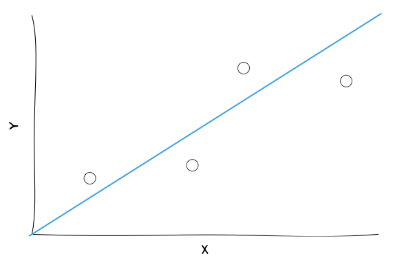
The problem:
We know that a straight line has the form \( Y=mX+b \)
What values of \( m \) and \( b \) are the “best”?
Curve Fitting Solution

The red lines indicate how far the fitted line is from the true data points.
Curve Fitting Solution

- \( (X_p, Y_p) \) is the real data
- \( {Y'}_p = mX_p+b \) gives us the predicted Y value for \( X_p \)
- The distance “missed by”
- \( Y_p-{Y'}_p= Y_p - (mX_p + b) \)
Curve Fitting Solution
Now calculate the sum of the squares of all the “misses”
\[ Sum= (Y_1 - (mX_1 + b))^2 + (Y_2 - (mX_2 + b))^2 + ...\\+...+ (Y_N - (mX_N + b))^2 \]
Note: All \( X_i \) and \( Y_i \) are known.
This becomes a calculus problem to select \( m \) and \( b \) that minimizes the sum.
Curve Fitting Solution
Calculate partial derivatives (pardon?), setting them equal to zero and solving.
\[ \bbox[5px, border:2px solid black]{m = \frac{N\sum_{i=1}^N X_i Y_i - \sum_{i=1}^N X_i \sum_{i=1}^N Y_i}{N \sum_{i=1}^N (X_i^2)-(\sum_{i=1}^N X_i)^2}} \]
\[ \bbox[5px, border:2px solid black]{b=\frac{\sum_{i=1}^N Y_i - m\sum_{i=1}^N X_i}{N}} \]
Common Concern
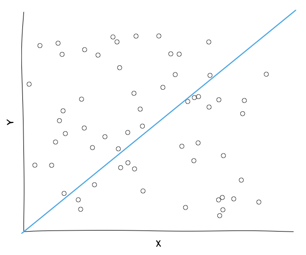
Given ANY set of data points, we can find \( m \) and \( b \). Is it always a good idea to do this?
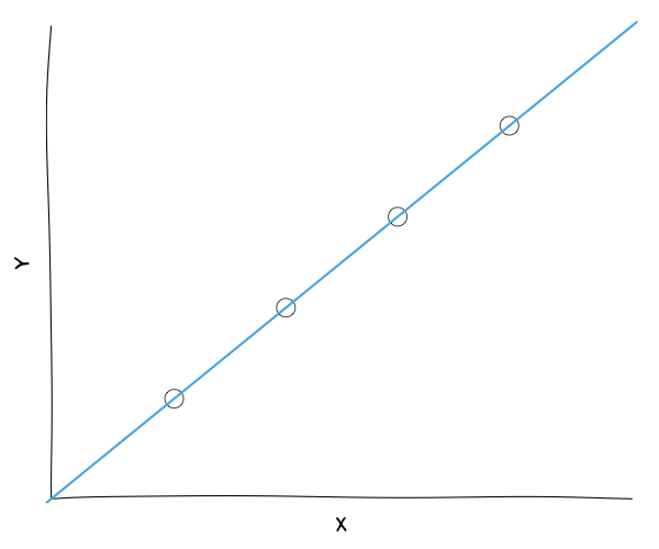
Common Concern
Given ANY set of data points, we can find \( m \) and \( b \). Is it always a good idea to do this?
Correlation Coefficient
\[ R= \frac{\sum_{i=1}^N \left [(X_i- \bar X)(Y_i- \bar Y) \right ]}{\left [\sum_{i=1}^{N}(X_i- \bar X)^2 \sum_{i=1}^{N}(Y_i- \bar Y)^2 \right ]^ { \frac{1}{2} }} \]
Correlation Coefficient
\[ R= \frac{\sum_{i=1}^N \left [(X_i- \bar X)(Y_i- \bar Y) \right ]}{\left [\sum_{i=1}^{N}(X_i- \bar X)^2 \sum_{i=1}^{N}(Y_i- \bar Y)^2 \right ]^ { \frac{1}{2} }} \]
\( -1 \le R \le 1 \)
- \( R=1 \ \) means perfect correlation
- \( R=0 \ \) means totally uncorrelated
- \( R=-1 \ \) means …
Alternative R
Note: an alternate equation for R is found as shown here
\[ \bbox[5px, border:2px solid black]{ R = \frac{n \left (\sum{x_i y_i} \right ) - \left (\sum x_i \right) \left (\sum y_i \right)}{\sqrt {n \left (\sum x_i^2 \right )- \left (\sum x_i \right )^2} \sqrt {n \left (\sum y_i^2 \right )- \left (\sum y_i \right)^2}} } \]
Suggestions
Anytime you do a linear regression (or other types of curve-fitting) you should check the correlation coefficient (or other goodness-of-fit parameters)
\[ Is \ R=0.9 \ good \ enough? \]
\[ How \ about \ R=0.8 ? \ 0.7? \]
Deciding if R is “good enough” is an interpretive skill developed through experience.
If \( R=0.8 \), then 64% of the variance in the dependent variable is explainable by the variance in the independent variable. Note: \( \ R^2 = 0.64 \)
Nonlinear Graphs
“Patterned” data not following a straight line?
Model with a curved line
Transform to a straight line model

Nonlinear Graphs: Power
Then,
\( V=bT^m \ \ \ \) ——> \( \ \ \log \ V=log \ b+ m \log \ T \)
i.e., Let \( Y=log \ V \) and \( X = log \ T \)
Now do a linear regression on the variables log T and log V. Note that the intercept derived is log b (NOT b)
Nonlinear Graphs: Exponential
Then,
\( V=be^{mt} \ \ \ \) ——> \( \ \ \log \ V=log \ b+ m t \)
i.e., Let \( Y=log \ V \) and \( X = t \)
Now do a linear regression on the variables t and log V. Note that the intercept derived is log b (NOT b)