Instance selection for model-based classifiers
Walter Bennette
04-15-2014
Follow along
Take away message
Model-based classifiers with improved accuracy can be created by learning from carefully selected instances.
1 / 68
Outline
- Motivation
- Methodology
- Experimental results
- Conclusion
2 / 68
Motivation
A model-based classifier is an abstraction of data used to make predictions
- Retail
- Healthcare
- Finance
Better classifiers are beneficial
- Make fewer missclassifications
- Gain useful knowledge when analyzing the classifier
3 / 68
Motivation
- Aspects of a training dataset may make it difficult to build/induce/learn an accurate classifier
4 / 68
Motivation
Classes may overlap
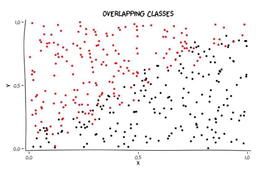
Where should these classes be separated?
5 / 68
Motivation
Classes may overlap
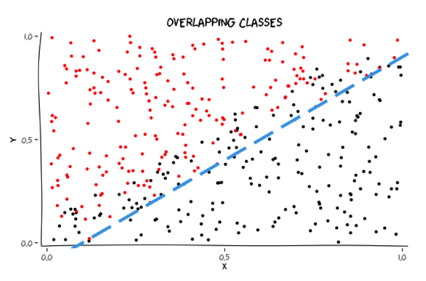
Where should these classes be separated?
5 / 68
Motivation
Classes may overlap
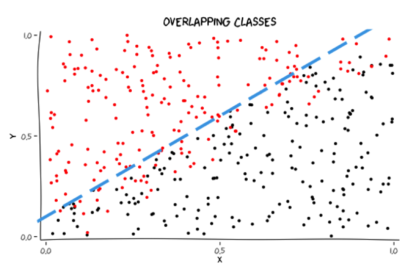
Where should these classes be separated?
5 / 68
Motivation
Classes may overlap
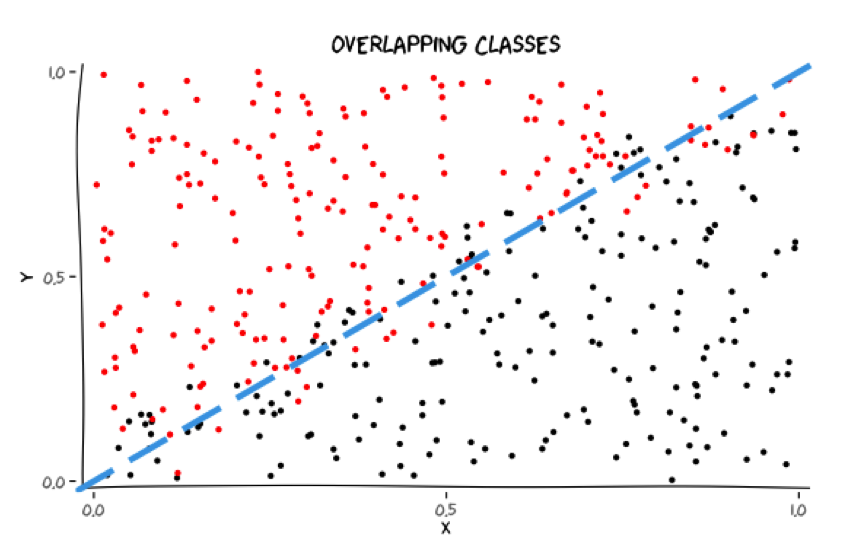
Where should these classes be separated?
5 / 68
Motivation
Classes may have outliers
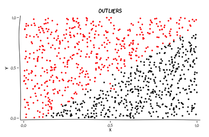
Should these outliers be accommodated?
6 / 68
Motivation
Classes may have outliers
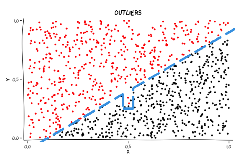
Should these outliers be accommodated?
6 / 68
Motivation
Minority class
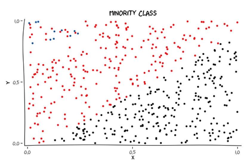
Does capturing the minority class introduce unnecessary structure?
7 / 68
Motivation
Minority class
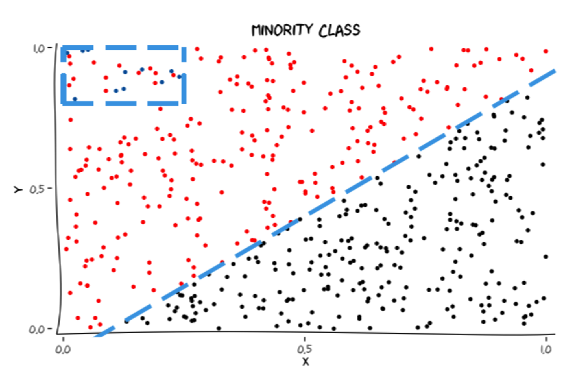
Does capturing the minority class introduce unnecessary structure?
7 / 68
Motivation
- We believe that selecting which instances to learn from can improve the accuracy of a classifier. This is called instance selection!
8 / 68
Outline
- Motivation
- Methodology
- Instance selection
- Previous work
- Integer programming formulation
- Instance selection
- Experimental results
- Conclusion
9 / 68
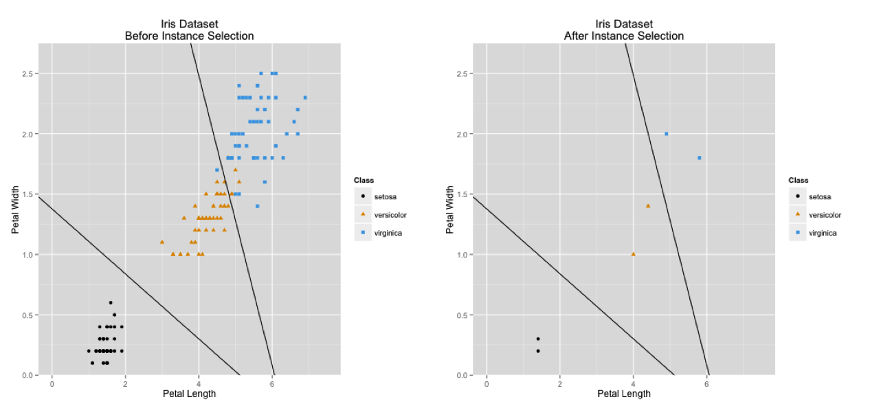
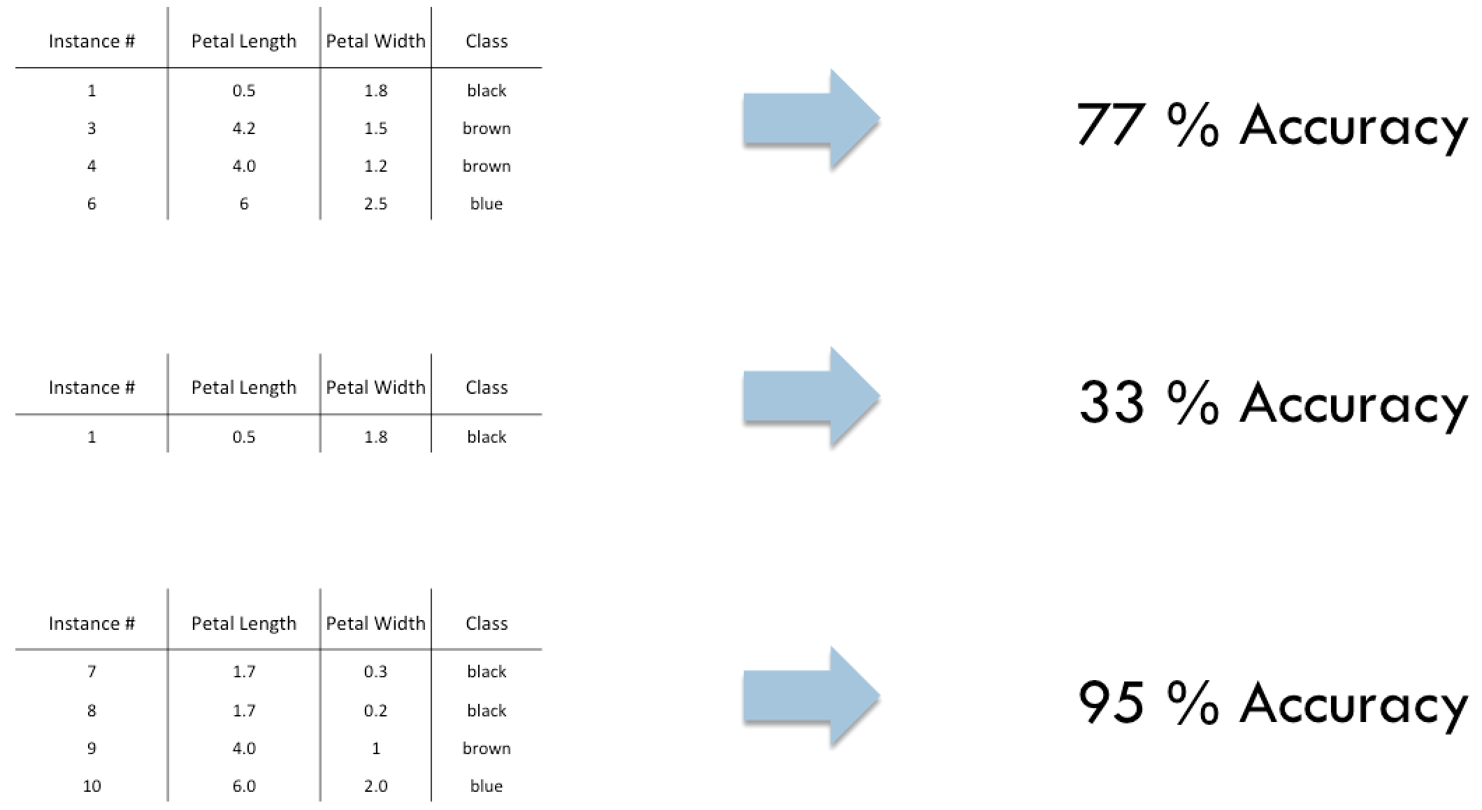
Instance selection
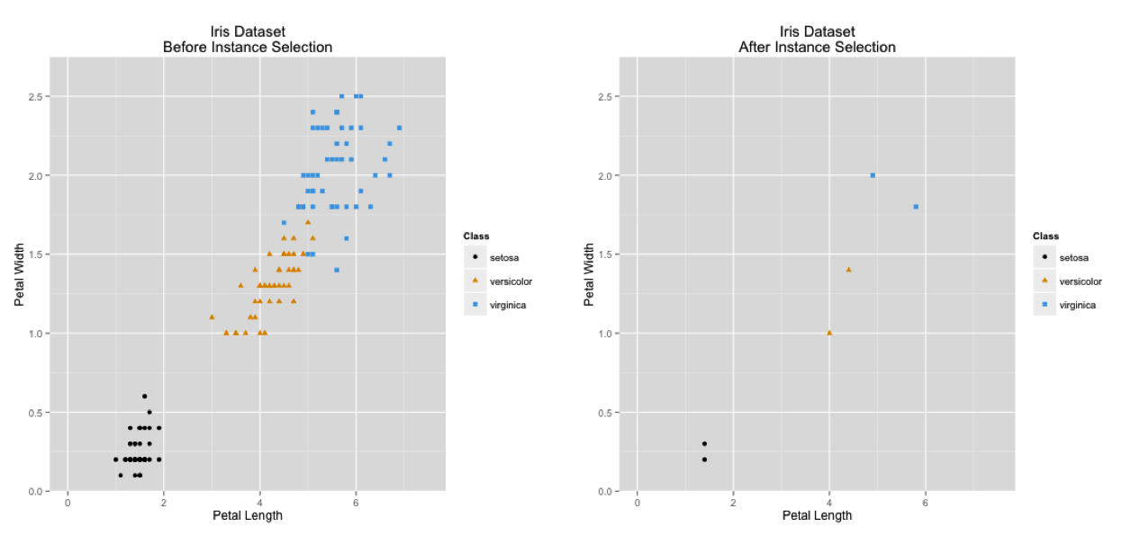
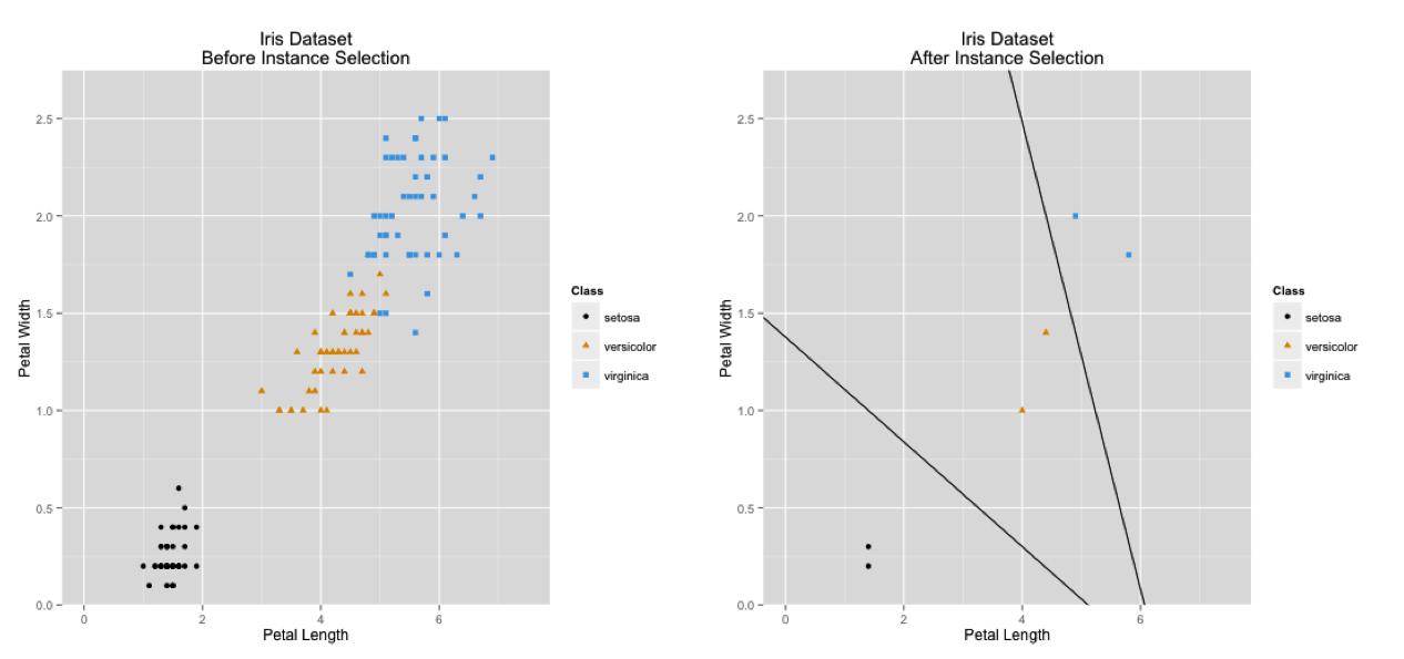
Instance selection addresses issues in the training data by creating a subset of the original data
The intention is that the classification algorithm will perform better when learning from the selected/reduced data set
10 / 68
Instance selection
11 / 68
Instance selection
11 / 68
Instance selection
11 / 68
Instance selection
12 / 68
Instance selection
- A combinatorial optimization problem (decide to include or not to include each instance)
- For a dataset of size \( n \) there are \( 2^n \) solutions
- There is no closed form objective function to maximize classifier accuracy
13 / 68
Outline
- Motivation
- Methodology
- Instance selection
- Previous work
- Integer programming formulation
- Instance selection
- Experimental results
- Conclusion
14 / 68
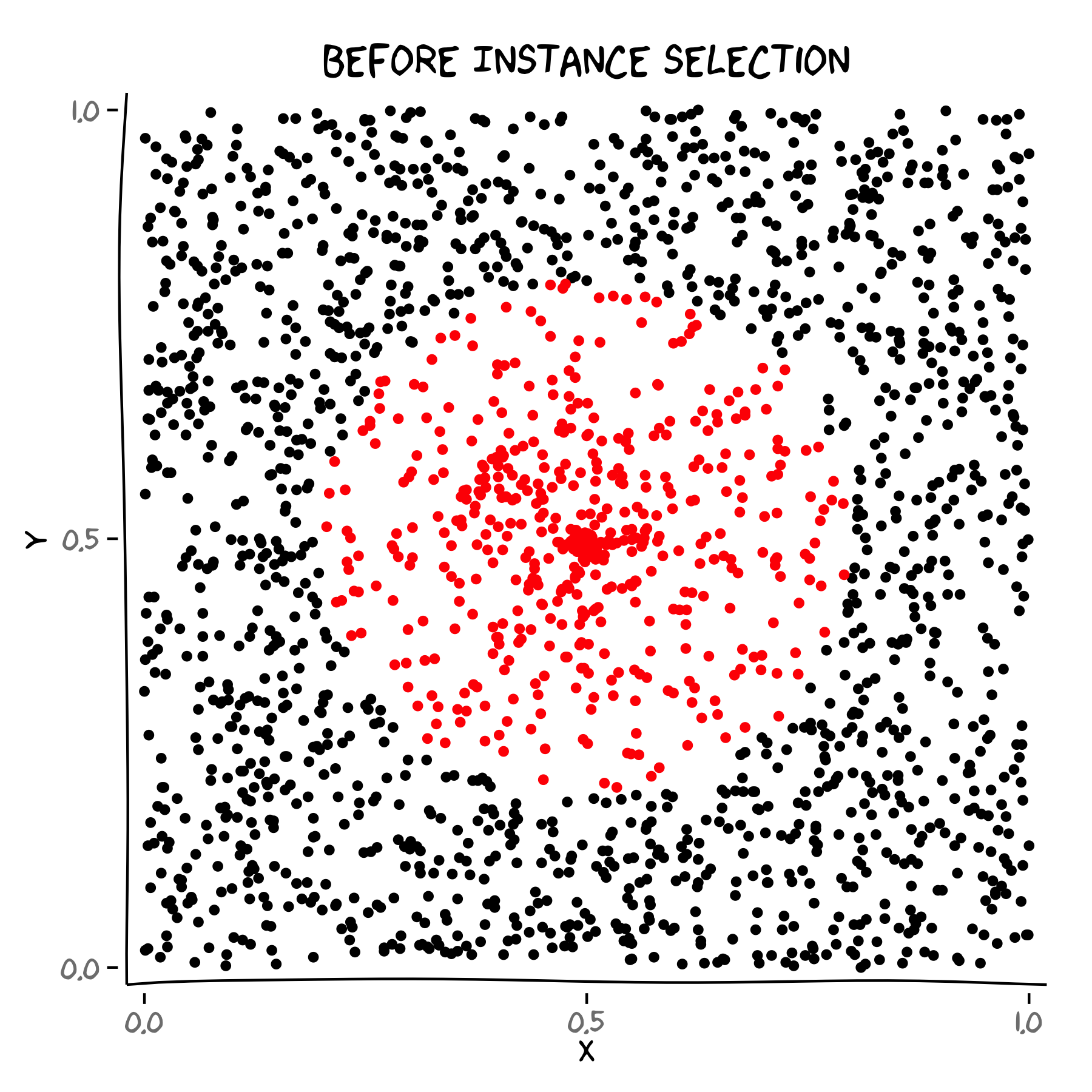
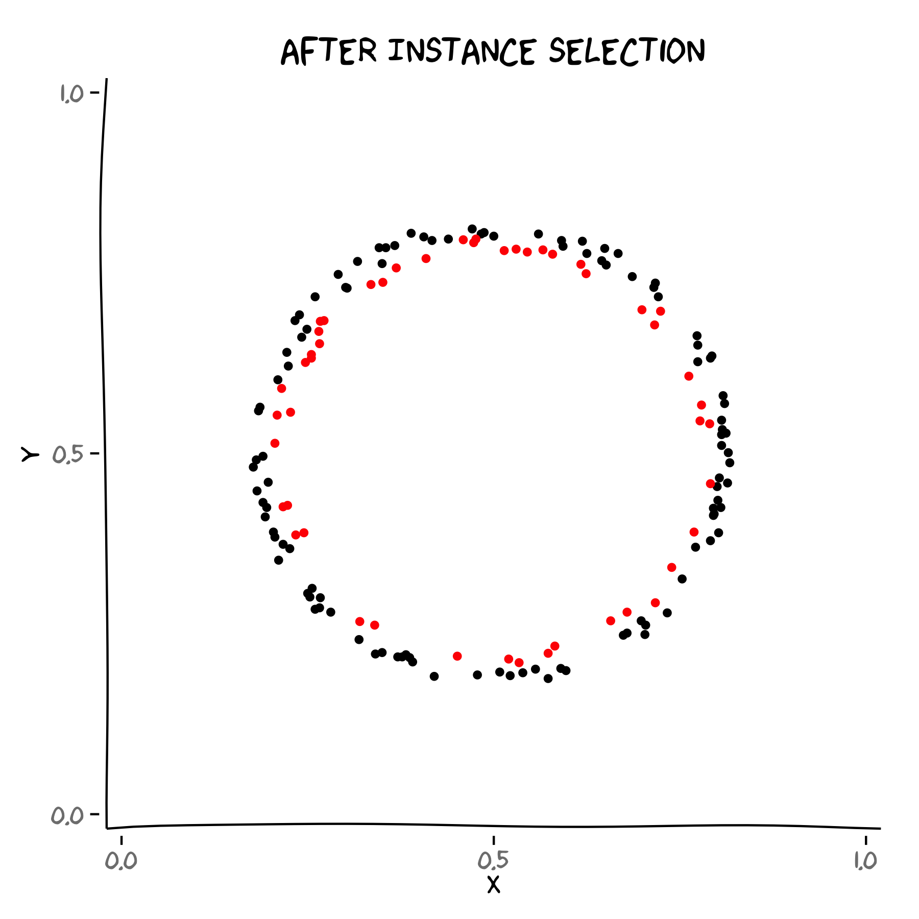
Previous work
Started for k-NN
15 / 68
Previous work
Made sense for model-based classifiers
\( {\mathbf {Max} \ \ \ \ Classifier \ Accuracy \\ \mathbf {s.t} \\ \ \ \ \ \ \ \ \ \ \ \ \ \ x_i \in \{0,1\} \ \forall \ i \in I} \)
- This is a combinatorial optimization problem
- There are \( 2^n \) possible solutions
- There is no closed form for the objective function
16 / 68
Previous work
A VAST majority rely on evolutionary algorithms to find a solution
Other optimization problems look similar to instance selection if the problem is reformulated. This allows us to take advantage of optimization theory.
17 / 68
Previous work
C. Reeves, S. Taylor, Selection of training sets for neural networks by a genetic algorithm, Parallel Problem Solving from Nature- PSSN V, (1998) 633-642.
C. Reeves, D Bush, Using genetic algorithms for training data selection in RBF networks, in: Instance Selection and Construction for Data Mining, H. Liu and H. Motoda (Eds), Kluwer, Norwell, MA, (2001) pp.339–356.
T. Endou, Q. Zhao, Generation of Comprehensible Decision Trees Through Evolution of Training Data, in proceedings of the 2002 Congress on Evolutionary Computation, (2002) 1221-1225.
J. Cano, F. Herrera, M. Lozano, Using Evolutionary Algorithms as Instance Selection for Data Reduction in KDD: An Experimental Study, IEEE Transactions on Evolutionary Computation, 7(6) (2003) 561-575.
J. Cano, F. Herrera, M. Lozano, Evolutionary Stratified Training Set Selection for Extracting Classification Rules with Trade off Precision-Interpretability, Data & Knowledge Engineering, 60 (2006) 90-108.
N. Garcia-Pedrajas, Evolutionary computation for training set selection, WIREs Data Mining and Knowledge Discovery, 1 (2011) 512-523.
Kim K-J, Artificial neural networks with evolutionary instance selection for financial forecasting, Expert Syst Appl, 30 (2006) 519-526.
Wu, Shuing. Optimal instance selection for improved decision tree. (2007 Dissertation)
Walter Bennette, Instance selection for simplified decision trees through the generation and selection of instance candidate subsets. (2009 Master’s thesis)
Walter Bennette, Sigurdur Olafsson, Model based classifier improvement through the generation and selection of instance candidate subsets, Data and Knowledge Engineering (under revision).
18 / 68
Outline
- Motivation
- Methodology
- Instance selection
- Previous work
- Integer programming formulation
- Instance selection
- Experimental results
- Conclusion
19 / 68
Integer programming formulation
New decision variables
- Should the \( j^{th} \) subset (column) of instances be included in the training data?
- \( x_j \in \{0,1\} \ \forall \ j \in J \)
- Example
- \( Training \ Data = \{\tau_1, \tau_2, ..., \tau_n \} \)
- \( Column^{(1)} = \{\tau_1, \tau_5, \tau_6 \} \)
- \( Column^{(1)} \ accuracy= c_1 \)
- \( \ If \ x_1 = 1, \ then \ \{\tau_1, \tau_5, \tau_6 \} \subseteq \ New \ Training \ Data \)
20 / 68
Integer programming formulation
Formulation 1
\( \mathbf {Max} \ \ \ \sum_{j \in J}c_jx_j \)
\( \mathbf {s.t} \)
\( \ \ \ \ \ \ \ \ \ \ \sum_{j \in J}a_{ij}x_j \le 1 \ \ \forall \ i \in I \)
\( \ \ \ \ \ \ \ \ \ \ \ x_j \in \{0,1\} \ \ \forall \ j \in J \)
21 / 68
Integer programming formulation
Formulation 1
\( \mathbf {Max} \ \ \ \sum_{j \in J}c_jx_j \)
\( \mathbf {s.t} \)
\( \ \ \ \ \ \ \ \ \ \ \sum_{j \in J}a_{ij}x_j \le 1 \ \ \forall \ i \in I \)
\( \ \ \ \ \ \ \ \ \ \ \ x_j \in \{0,1\} \ \ \forall \ j \in J \)
<—A column is
associated with each
possible subset of
instances
21 / 68
Integer programming formulation
Formulation 1
\( \mathbf {Max} \ \ \ \sum_{j \in J}c_jx_j \)
\( \mathbf {s.t} \)
\( \ \ \ \ \ \ \ \ \ \ \sum_{j \in J}a_{ij}x_j \le 1 \ \ \forall \ i \in I \)
\( \ \ \ \ \ \ \ \ \ \ \ x_j \in \{0,1\} \ \ \forall \ j \in J \)
<— \( a_{ij} \) indicates if instance
\( i \ \) is in column \( \ j \)
21 / 68
Integer programming formulation
Formulation 1
\( \mathbf {Max} \ \ \ \sum_{j \in J}c_jx_j \)
\( \mathbf {s.t} \)
\( \ \ \ \ \ \ \ \ \ \ \sum_{j \in J}a_{ij}x_j \le 1 \ \ \forall \ i \in I \)
\( \ \ \ \ \ \ \ \ \ \ \ x_j \in \{0,1\} \ \ \forall \ j \in J \)
<— \( c_j \) is the accuracy of a
classifier built from
the contents in column
\( \ j \)
21 / 68
Integer programming formulation
Example
\( Training= \{\tau_1, \tau_2\} \)
\( Column^{(1)}=\{\ \} \)
\( Column^{(2)}=\{\tau_1 \} \)
\( Column^{(3)}=\{\tau_2 \} \)
\( Column^{(4)}=\{\tau_1, \tau_2 \} \)
\( \mathbf {Max} \ \ \ \ 0.3x_1 + 0.7x_2 + 0.5x_3 + 0.6x_4 \)
\( \mathbf {s.t} \)
\( \ \ \ \ \ \ \ \ \ \ \ \ 0x_1 + 1x_2 + 0x_3 + 1x_4 \le 1 \)
\( \ \ \ \ \ \ \ \ \ \ \ \ 0x_1 + 0x_2 + 1x_3 + 1x_4 \le 1 \)
\( \ \ \ \ \ \ \ \ \ \ \ \ x_1, x_2, x_3, x_4 \in \{0,1\} \)
22 / 68
Integer programming formulation
Formulation 2
\( \mathbf {Max} \ \ \ \sum_{j \in J}c_jx_j \)
\( \mathbf {s.t} \)
\( \ \ \ \ \ \ \ \ \ \ \sum_{j \in J}x_j \le 1 \)
\( \ \ \ \ \ \ \ \ \ \ \ x_j \in \{0,1\} \ \ \forall \ j \in J \)
23 / 68
Integer programming formulation
Formulation 2
\( \mathbf {Max} \ \ \ \sum_{j \in J}c_jx_j \)
\( \mathbf {s.t} \)
\( \ \ \ \ \ \ \ \ \ \ \sum_{j \in J}x_j \le 1 \)
\( \ \ \ \ \ \ \ \ \ \ \ x_j \in \{0,1\} \ \ \forall \ j \in J \)
<—A column is
associated with each
possible subset of
instances
23 / 68
Integer programming formulation
Formulation 2
\( \mathbf {Max} \ \ \ \sum_{j \in J}c_jx_j \)
\( \mathbf {s.t} \)
\( \ \ \ \ \ \ \ \ \ \ \sum_{j \in J}x_j \le 1 \)
\( \ \ \ \ \ \ \ \ \ \ \ x_j \in \{0,1\} \ \ \forall \ j \in J \)
<— Select at most one
column
23 / 68
Integer programming formulation
Formulation 2
\( \mathbf {Max} \ \ \ \sum_{j \in J}c_jx_j \)
\( \mathbf {s.t} \)
\( \ \ \ \ \ \ \ \ \ \ \sum_{j \in J}x_j \le 1 \)
\( \ \ \ \ \ \ \ \ \ \ \ x_j \in \{0,1\} \ \ \forall \ j \in J \)
<— \( c_j \) is the accuracy of a
classifier built from
the contents of
column \( \ j \)
23 / 68
Integer programming formulation
Example
\( Training= \{\tau_1, \tau_2\} \)
\( Column^{(1)}=\{\ \} \)
\( Column^{(2)}=\{\tau_1 \} \)
\( Column^{(3)}=\{\tau_2 \} \)
\( Column^{(4)}=\{\tau_1, \tau_2 \} \)
\( \mathbf {Max} \ \ \ \ 0.3x_1 + 0.7x_2 + 0.5x_3 + 0.6x_4 \)
\( \mathbf {s.t} \)
\( \ \ \ \ \ \ \ \ \ \ \ \ x_1 + x_2 + x_3 + x_4 \le 1 \)
\( \ \ \ \ \ \ \ \ \ \ \ \ x_1, x_2, x_3, x_4 \in \{0,1\} \)
24 / 68
Integer programming formulation
Issue
For Formulation 1 and Formulation 2, a dataset of size \( n \) has \( 2^n \) columns
Solution
1. Begin with a good set of initial columns
2. Use column generation to find improvements
25 / 68
Outline
- Motivation
- Methodology
- Instance selection
- Previous work
- Integer programming formulation
- Column generation
- An approximation
- Column generation
- Instance selection
- Experimental results
- Conclusion
26 / 68
Column generation
\( Training \ \ = \{\tau_1, \tau_2, \tau_3 \} \)
\( Column^{(2)} = \{ \tau_1 \} \)
\( Column^{(6)} = \{ \tau_1, \tau_3 \} \)
\( \mathbf {Max} \ \ \ \ 0.6x_2 + 0.7x_6 \)
\( \mathbf {s.t} \)
\( \ \ \ \ \ \ \ \ \ \ \ \ 1x_2 + 1x_6 \le 1 \)
\( \ \ \ \ \ \ \ \ \ \ \ \ 0x_2 + 0x_6 \le 1 \)
\( \ \ \ \ \ \ \ \ \ \ \ \ 0x_2 + 1x_6 \le 1 \)
\( \ \ \ \ \ \ \ \ \ \ \ \ 0 \le x_2, x_6 \)
27 / 68
Column generation
\( Training \ \ = \{\tau_1, \tau_2, \tau_3 \} \)
\( Column^{(2)} = \{ \tau_1 \} \)
\( Column^{(6)} = \{ \tau_1, \tau_3 \} \)
\( \mathbf {Max} \ \ \ \ 0.6x_2 + 0.7x_6 \)
\( \mathbf {s.t} \)
\( \ \ \ \ \ \ \ \ \ \ \ \ 1x_2 + 1x_6 \le 1 \)
\( \ \ \ \ \ \ \ \ \ \ \ \ 0x_2 + 0x_6 \le 1 \)
\( \ \ \ \ \ \ \ \ \ \ \ \ 0x_2 + 1x_6 \le 1 \)
\( \ \ \ \ \ \ \ \ \ \ \ \ 0 \le x_2, x_6 \)
—> Solve and get dual
variables
27 / 68
Column generation
\( Training \ \ = \{\tau_1, \tau_2, \tau_3 \} \)
\( Column^{(2)} = \{ \tau_1 \} \)
\( Column^{(6)} = \{ \tau_1, \tau_3 \} \)
\( \mathbf {Max} \ \ \ \ 0.6x_2 + 0.7x_6 \)
\( \mathbf {s.t} \)
\( \ \ \ \ \ \ \ \ \ \ \ \ 1x_2 + 1x_6 \le 1 \)
\( \ \ \ \ \ \ \ \ \ \ \ \ 0x_2 + 0x_6 \le 1 \)
\( \ \ \ \ \ \ \ \ \ \ \ \ 0x_2 + 1x_6 \le 1 \)
\( \ \ \ \ \ \ \ \ \ \ \ \ 0 \le x_2, x_6 \)
—> \( \pi^*=\{0.6, 0, 0.1\} \)
27 / 68
Column generation
Price out problem
\( \mathbf {Max} \ \ \ \ c^{new} - \pi^*a^{new} \)
\( \mathbf {s.t} \)
\( \ \ \ \ \ \ \ \ \ \ \sum_{i \in I} a_i^{new} \le G \)
\( \ \ \ \ \ \ \ \ \ \ \ a_i^{new} \in \{0,1\} \ \forall i \in I \)
28 / 68
Column generation
Price out problem
\( \mathbf {Max} \ \ \ \ c^{new} - (0.6a_1+0a_2+0.1a_3) \)
\( \mathbf {s.t} \)
\( \ \ \ \ \ \ \ \ \ \ \ \ a_1 + a_2 + a_3\le 3 \)
\( \ \ \ \ \ \ \ \ \ \ \ \ a_1, a_2, a_3 \in \{0,1\} \)
| Column | \( a_1 \) | \( a_2 \) | \( a_3 \) | \( c^{new} \) |
|---|---|---|---|---|
| \( Column^{(1)} \) | 0 | 0 | 0 | 0.30 |
| \( Column^{(3)} \) | 0 | 1 | 0 | 0.60 |
| \( Column^{(4)} \) | 0 | 0 | 1 | 0.60 |
| \( Column^{(5)} \) | 1 | 1 | 0 | 0.50 |
| \( Column^{(7)} \) | 0 | 1 | 1 | 0.70 |
| \( Column^{(8)} \) | 1 | 1 | 1 | 0.70 |
29 / 68
Column generation
Price out problem
\( \mathbf {Max} \ \ \ \ c^{new} - (0.6a_1+0a_2+0.1a_3) \)
\( \mathbf {s.t} \)
\( \ \ \ \ \ \ \ \ \ \ \ \ a_1 + a_2 + a_3\le 3 \)
\( \ \ \ \ \ \ \ \ \ \ \ \ a_1, a_2, a_3 \in \{0,1\} \)
| Column | \( a_1 \) | \( a_2 \) | \( a_3 \) | \( c^{new} \) | Obj |
|---|---|---|---|---|---|
| \( Column^{(1)} \) | 0 | 0 | 0 | 0.30 | 0.30 |
| \( Column^{(3)} \) | 0 | 1 | 0 | 0.60 | 0.60 |
| \( Column^{(4)} \) | 0 | 0 | 1 | 0.60 | 0.50 |
| \( Column^{(5)} \) | 1 | 1 | 0 | 0.50 | -0.10 |
| \( Column^{(7)} \) | 0 | 1 | 1 | 0.70 | 0.60 |
| \( Column^{(8)} \) | 1 | 1 | 1 | 0.70 | 0.00 |
29 / 68
Column generation
\( Training \ \ = \{\tau_1, \tau_2, \tau_3 \} \)
\( Column^{(2)} = \{ \tau_1 \} \)
\( Column^{(6)} = \{ \tau_1, \tau_3 \} \)
\( Column^{(3)} = \{ \tau_2 \} \)
\( \mathbf {Max} \ \ \ \ 0.6x_2 + 0.7x_6 + 0.6x_3 \)
\( \mathbf {s.t} \)
\( \ \ \ \ \ \ \ \ \ \ \ \ 1x_2 + 1x_6 + 0x_3\le 1 \)
\( \ \ \ \ \ \ \ \ \ \ \ \ 0x_2 + 0x_6 +1x_3\le 1 \)
\( \ \ \ \ \ \ \ \ \ \ \ \ 0x_2 + 1x_6 +0x_3\le 1 \)
\( \ \ \ \ \ \ \ \ \ \ \ \ 0 \le x_1, x_2, x_3 \)
30 / 68
Column generation
\( Training \ \ = \{\tau_1, \tau_2, \tau_3 \} \)
\( Column^{(2)} = \{ \tau_1 \} \)
\( Column^{(6)} = \{ \tau_1, \tau_3 \} \)
\( Column^{(3)} = \{ \tau_2 \} \)
\( \mathbf {Max} \ \ \ \ 0.6x_2 + 0.7x_6 + 0.6x_3 \)
\( \mathbf {s.t} \)
\( \ \ \ \ \ \ \ \ \ \ \ \ 1x_2 + 1x_6 + 0x_3\le 1 \)
\( \ \ \ \ \ \ \ \ \ \ \ \ 0x_2 + 0x_6 +1x_3\le 1 \)
\( \ \ \ \ \ \ \ \ \ \ \ \ 0x_2 + 1x_6 +0x_3\le 1 \)
\( \ \ \ \ \ \ \ \ \ \ \ \ 0 \le x_1, x_2, x_3 \)
—> Column generation can
continue until the
optimal solution is found
30 / 68
Outline
- Motivation
- Methodology
- Instance selection
- Previous work
- Integer programming formulation
- Column generation
- An approximation
- Column generation
- Instance selection
- Experimental results
- Conclusion
31 / 68
An approximation (or two)
From the price out problem:
\( \mathbf {Max} \ \ \ \ c^{new} - \pi^*a^{new} \)
An approximation of \( c^{new} \) based on \( a^{new} \) is necessary to implement column generation
32 / 68
An approximation (or two)
From the price out problem:
\( \mathbf {Max} \ \ \ \ c^{new} - \pi^*a^{new} \)
An approximation of classifier accuracy based on the contents of its training data is necessary to implement column generation
32 / 68
An approximation (or two)
Two approximations are developed. Each creates a ranking of the instances and assumes columns with high ranking instances will have high accuracy.
33 / 68
An approximation (or two)
Frequency approximation:
- Consider existing columns
- Identify columns with high accuracy
- Count the occurrences of instances in those columns
High ranking instances are those that appear frequently
34 / 68
An approximation (or two)
Information approximation:
\( L_{\tau} = - \sum_{j=1}^{|y|} P \left( y_j|\tau \right) log \left(P_E \left(y_j|\tau \right) \right) \)
- 0 for instances the classifier has mastered
- High for troubling instances
- 0 for instances the classifier has mastered
\[ Bh_{\tau} = \begin{cases} \ \ 0.1^{L_\tau}, & \text{if the classifier correctly classifies $\tau$} \\ (-0.1)^{L_\tau}, & \text{otherwise} \\ \end{cases} \]
- 1 means the classifier is great at classifying the instance
- 0 means it is confused
- -1 means it is horrible
35 / 68
An approximation (or two)
Information approximation:
- Build classifier from all the instances, calculate and sum \( Bh \)
- Build classifier from a subset of the instances, calculate and sum \( Bh \)
- Attribute the difference between the two to the missing instances
High ranking instances are those that decrease the value of \( Bh \)
36 / 68
An approximation (or two)
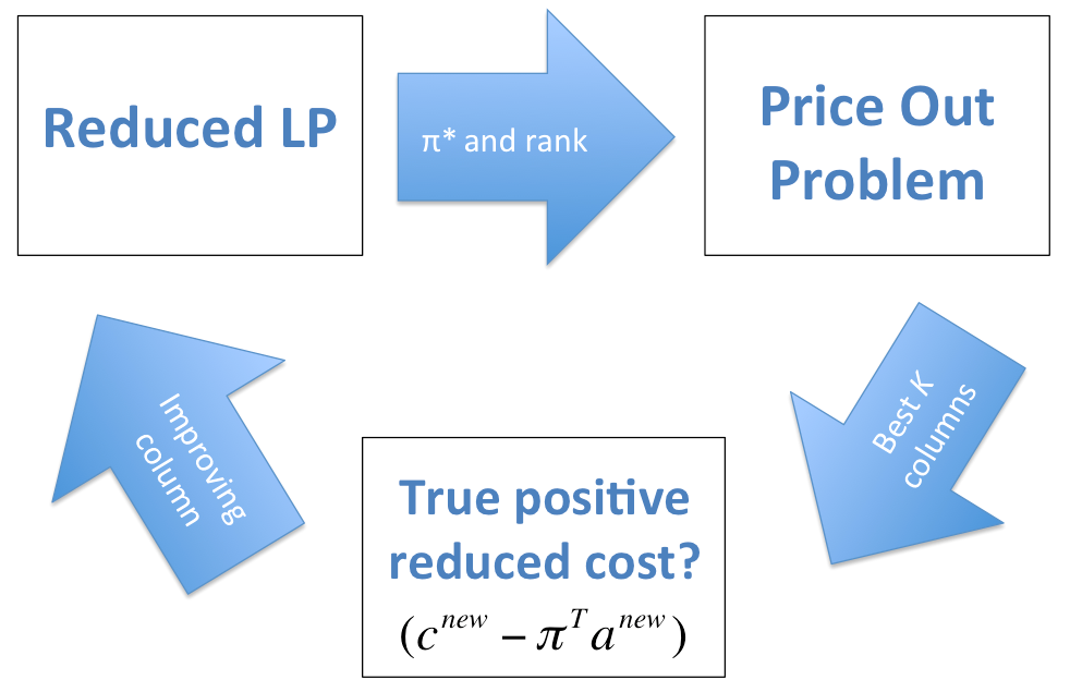
37 / 68
An approximation (or two)

A greedy selection procedure is used to combine columns into a final selection of instances
37 / 68
Integer programming formulation
Formulation 1
\( \mathbf {Max} \ \ \ \sum_{j \in J}c_jx_j \)
\( \mathbf {s.t} \)
\( \ \ \ \ \ \ \ \ \ \ \sum_{j \in J}a_{ij}x_j \le 1 \ \ \forall \ i \in I \)
\( \ \ \ \ \ \ \ \ \ \ \ x_j \in \{0,1\} \ \ \forall \ j \in J \)
Encourages the discovery of columns that have similar instances but higher accuracy
38 / 68
Integer programming formulation
Formulation 2
\( \mathbf {Max} \ \ \ \sum_{j \in J}c_jx_j \)
\( \mathbf {s.t} \)
\( \ \ \ \ \ \ \ \ \ \ \sum_{j \in J}x_j \le 1 \)
\( \ \ \ \ \ \ \ \ \ \ \ x_j \in \{0,1\} \ \ \forall \ j \in J \)
Discovers columns that have higher accuracy than any previously discovered column
39 / 68
Outline
- Motivation
- Methodology
- Experimental results
- Overall results
- Overfitting
- Successes
- Case study
- Overall results
- Conclusion
40 / 68
Overall Results
| Name | Instances | Attributes | Numeric | Nominal | Classes |
|---|---|---|---|---|---|
| Balance | 625 | 4 | Yes | No | 3 |
| Credit | 690 | 15 | Yes | Yes | 2 |
| Diabetes | 768 | 8 | Yes | No | 2 |
| Ecoli | 336 | 7 | Yes | No | 8 |
| Glass | 214 | 9 | Yes | No | 6 |
| Horse | 368 | 21 | Yes | Yes | 3 |
| Ionosphere | 351 | 34 | Yes | No | 2 |
| LandSat* | 444 | 36 | Yes | No | 6 |
| Spect | 267 | 22 | No | Yes | 2 |
| Tic-tac-toe | 958 | 9 | No | Yes | 2 |
| Waveform | 800 | 21 | Yes | No | 3 |
| Wisc Cancer | 699 | 9 | Yes | No | 2 |
41 / 68
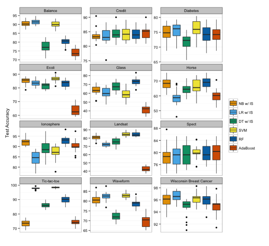
Overall Results
Instance selection is performed for:
- Naive Bayes (NB)
- Logistic Regression (LR)
- Decision Tree (DT)
Approach:
- 20 replications
- Paired-t test for difference of accuracy before and after instance selection
42 / 68
Overall Results
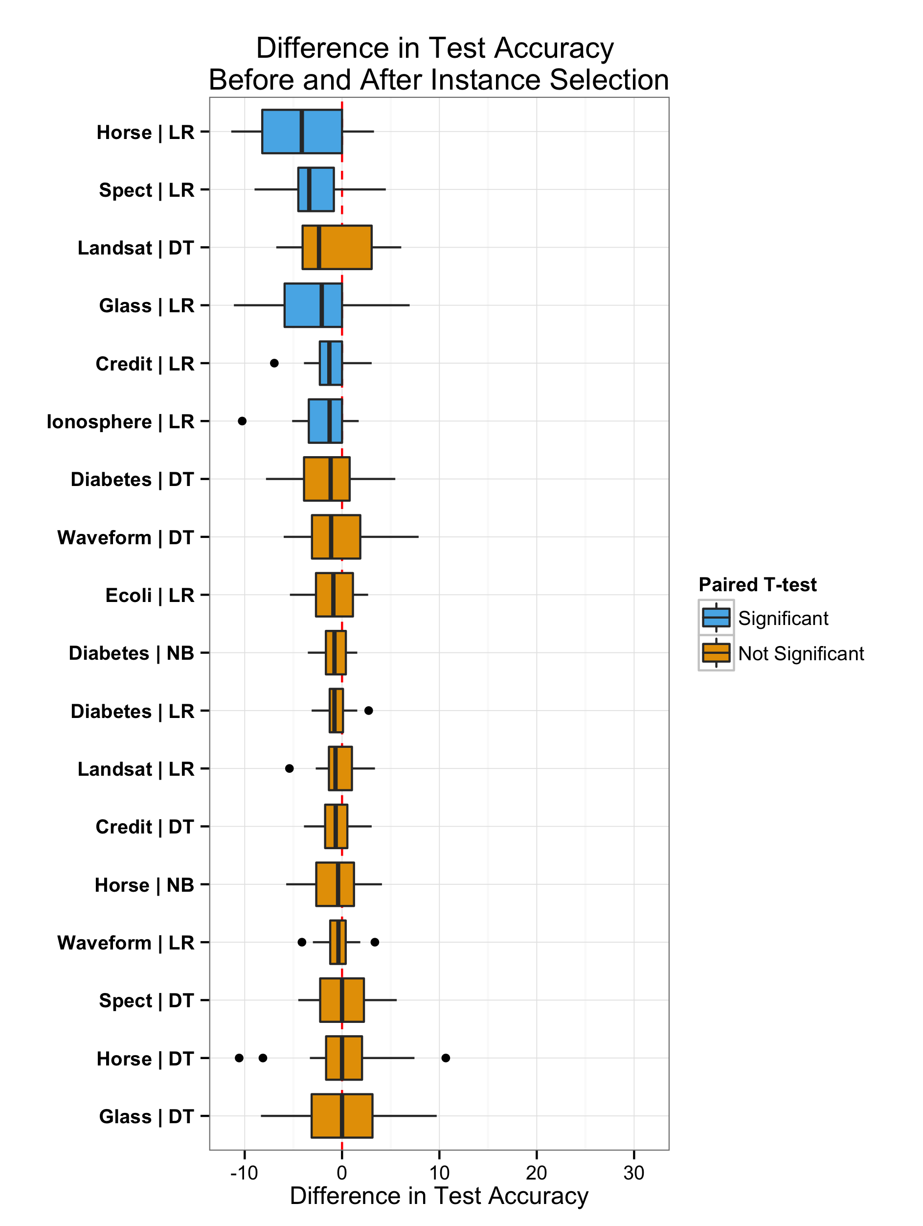
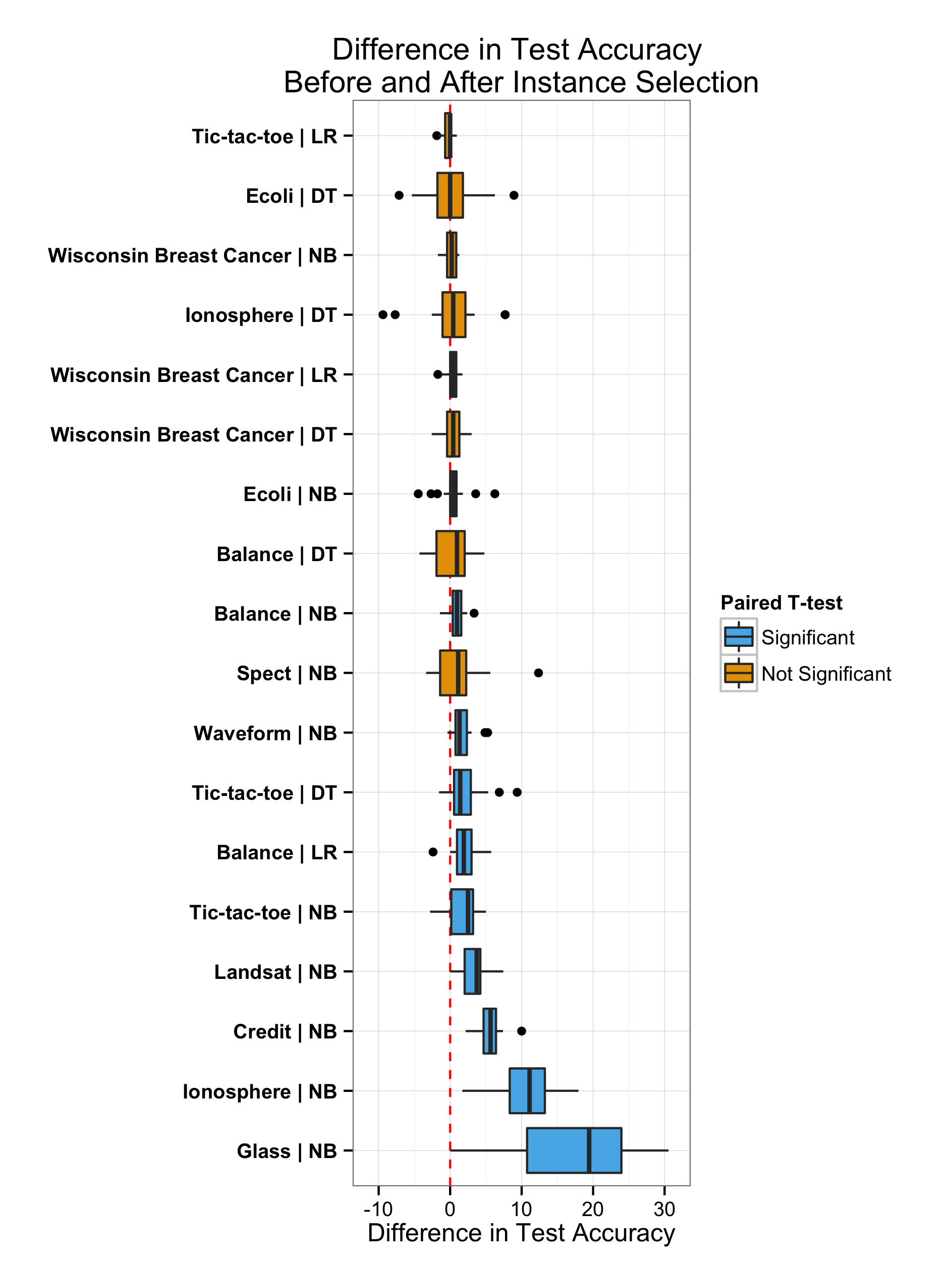
Outline
- Motivation
- Methodology
- Experimental results
- Overall results
- Overfitting
- Successes
- Case study
- Conclusion
44 / 68
Overfitting
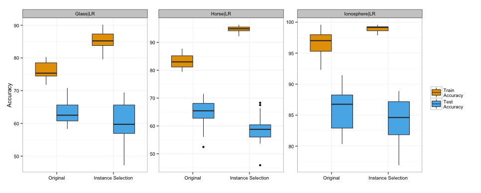
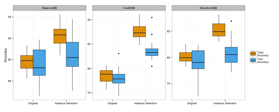
45 / 68
Overfitting
46 / 68
Outline
- Motivation
- Methodology
- Experimental results
- Overall results
- Overfitting
- Successes
- Case study
- Conclusion
47 / 68
Successes
The selected instances depend on
- The classifier
- The data
Instance selection is used as a wrapper
- Outliers?
- Overlapping classes?
- Minority classes?
48 / 68
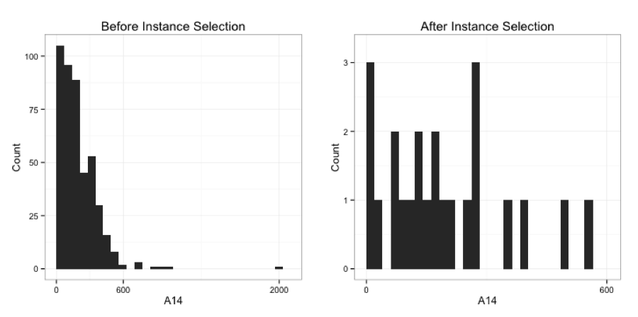
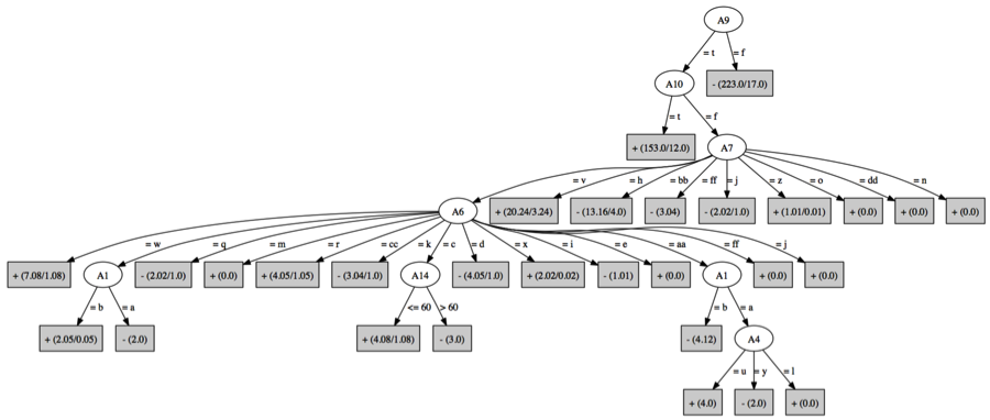
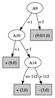
Credit dataset
- Classify customers as having good or bad credit
- Naive Bayes gained on average 5 percentage points
Instances with extreme values were removed
49 / 68
Credit dataset
50 / 68
Credit dataset
51 / 68
Credit dataset
52 / 68
Credit dataset
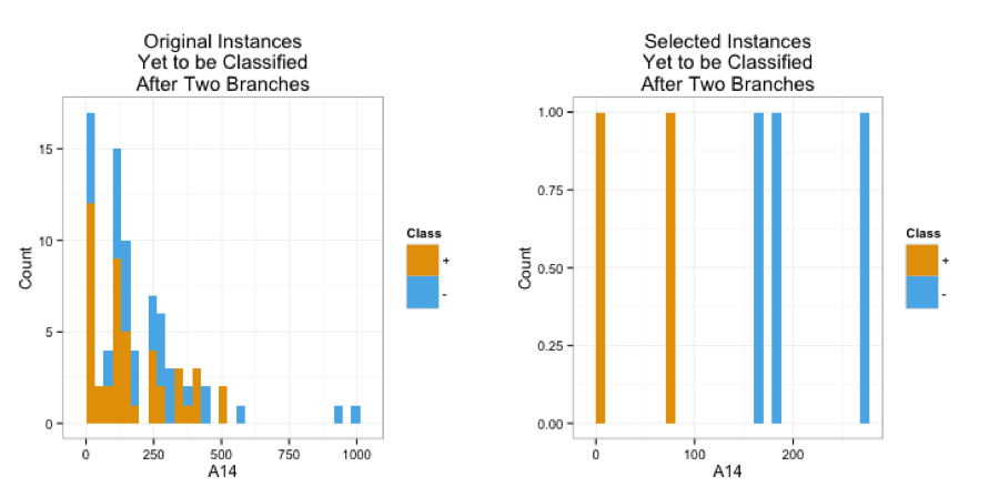
- Allowed naive Bayes to focus on the majority of the instances
- Perhaps benefitted from the easy to find seperation in A14 after instance selection
53 / 68
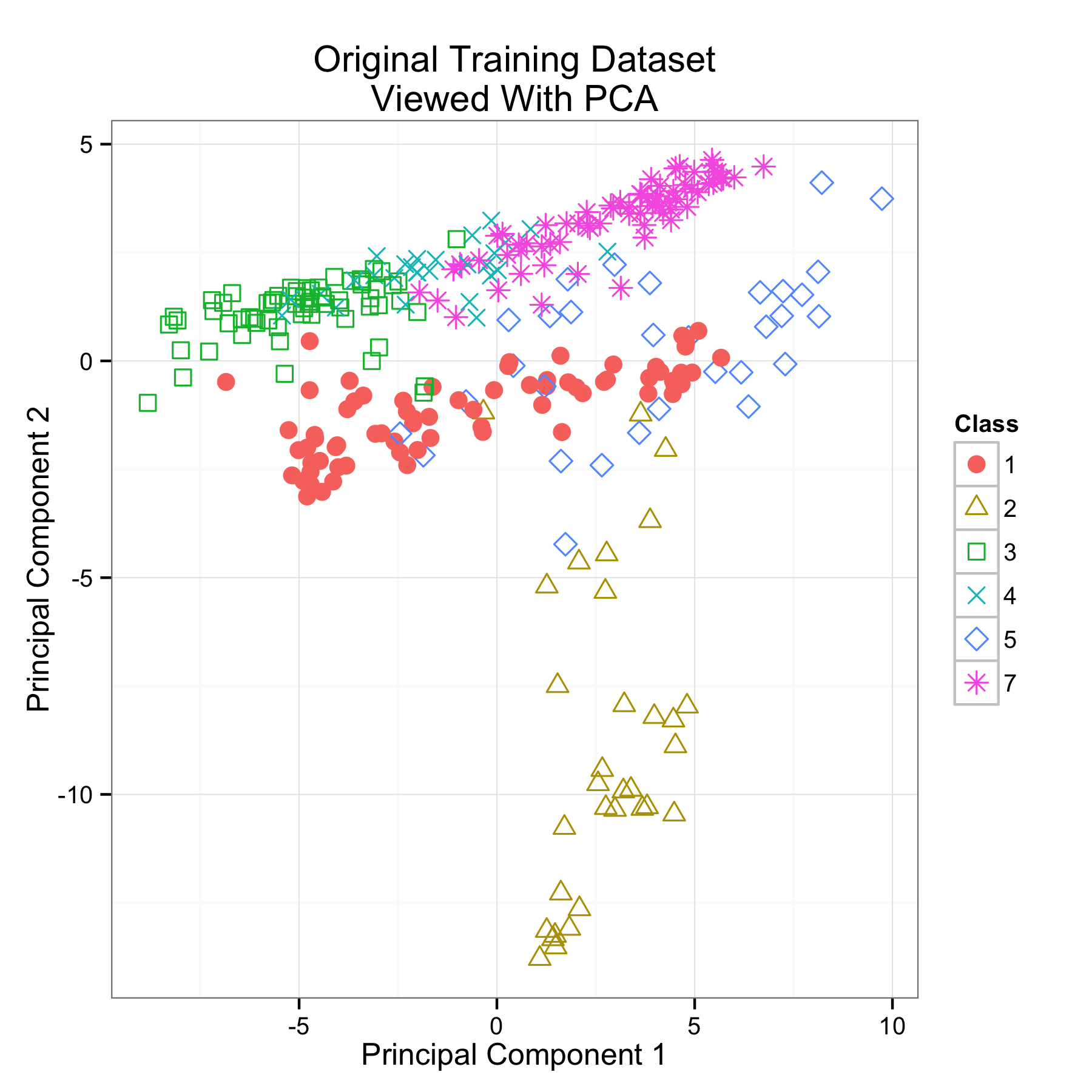
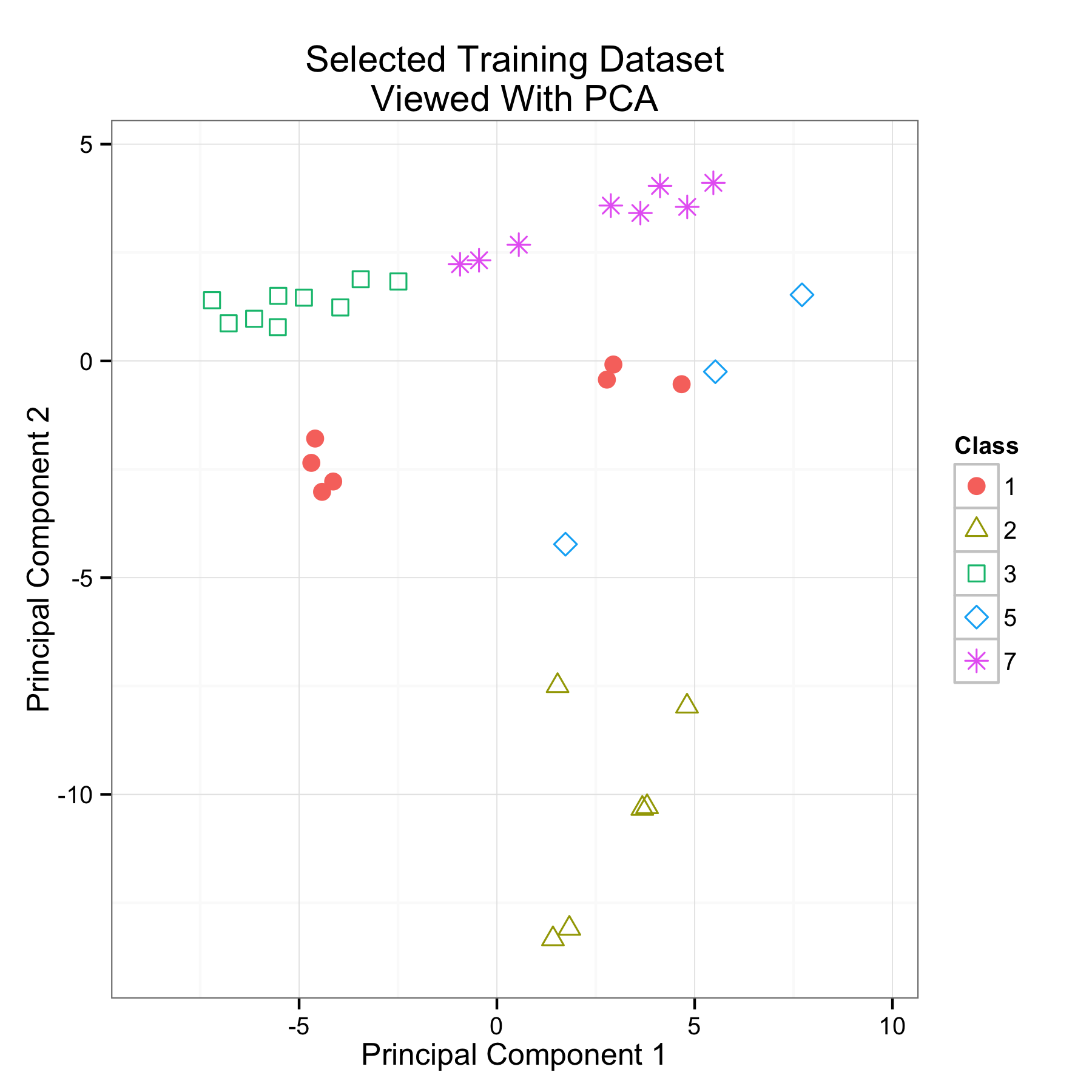
Landsat dataset
- Classify pixels of an image
- Logistic regression improved from 65% to 80%
54 / 68
Landsat dataset
55 / 68
Landsat dataset
56 / 68 Number of test instances misclassified
| Class1 | Class2 | Class3 | Class4 | Class5 | Class6 | Total | |
|---|---|---|---|---|---|---|---|
| Original Training Data | 5 | 9 | 11 | 9 | 8 | 9 | 51 |
| With Instance Selection | 1 | 3 | 3 | 14 | 5 | 2 | 28 |
- The ability to classify the minority class 4 is likely sacrificed in an effort to make it easier to separate the remaining classes
Successes
57 / 68
Outline
- Motivation
- Methodology
- Experimental results
- Overall results
- Overfitting
- Successes
- Case study
- Conclusion
58 / 68
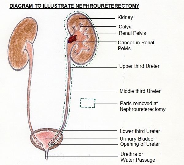
Case study
A Population-based Assessment of Perioperative Mortality After Nephroureterectomy for Upper-tract Urothelial Carcinoma
(I'll be calling this NU for UTUC!!)
59 / 68
Case study
Case study
Data: SEER database
Attributes: age, gender, histopathology, extraglandular
involvement, tumor grade, tumor size, and
mortality
Patients: 2,328 (9% mortality)
Classification task: predict mortality
Classifier: logistic regression
61 / 68
Case study
Confusion matrix of test data before instance selection
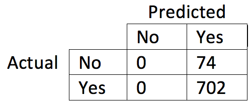
- 90% test accuracy
- Uninformative!
- Can use instance selection to maximize class balance accuracy
62 / 68
Case study
Confusion matrix of test data after instance selection
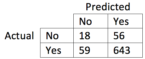
- 88% test accuracy
- Learn something about mortality
63 / 68
Case study
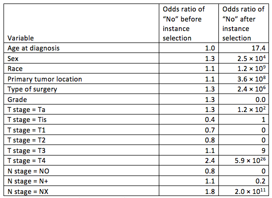
64 / 68
Outline
- Motivation
- Methodology
- Experimental results
- Conclusion
65 / 68
Conclusion
Reformulated instance selection as an integer program
Model-based classifiers with improved accuracy can be created by learning from carefully selected instances (because classifiers are imperfect)
Instance selection is useful for actual classification problems and is a competitive technique
66 / 68
Future work
Obvious
- Improve classifier accuracy estimate
- Address overfitting
- Accommodate bigger datasets
Interesting
- Optimize other metrics
- Imbalanced data
- Model simplicity
- Imbalanced data
67 / 68
Questions?
Walter Bennette
bennette@iastate.edu
68 / 68
Extras (SVM)
e1071
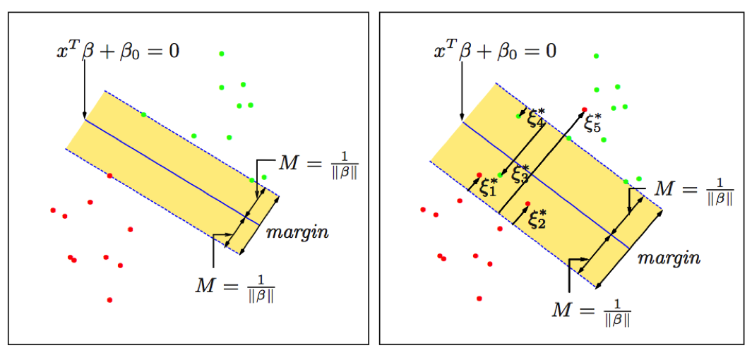
Extras (Wisconsin Breast Cancer)
train SVM: 98%
test SVM: 95%
train NB/IS: 98%
test NB/IS: 95%
Extras (Wisconsin Breast Cancer)
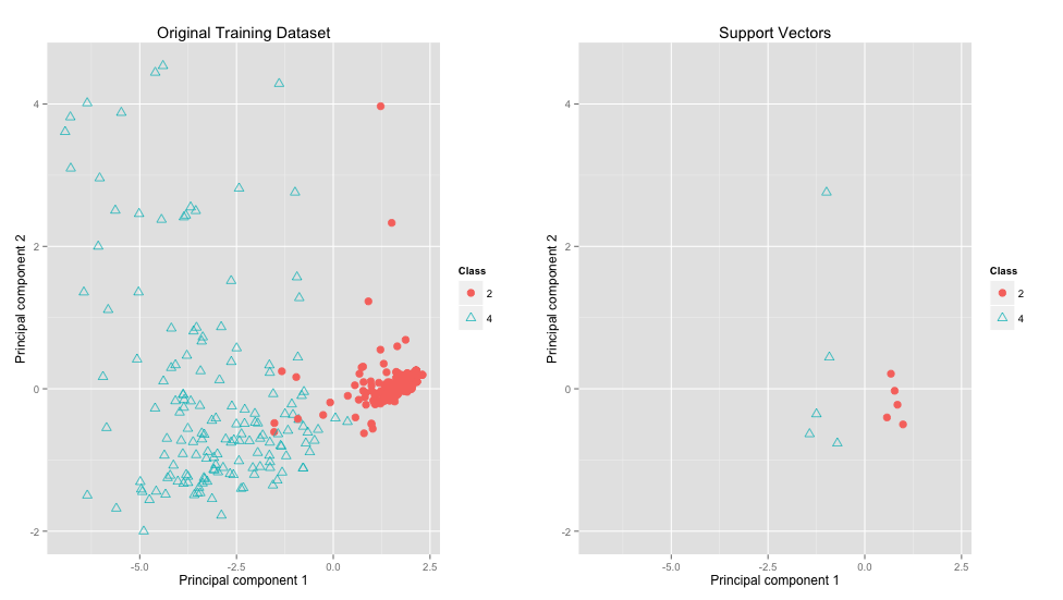
Extras (Wisconsin Breast Cancer)
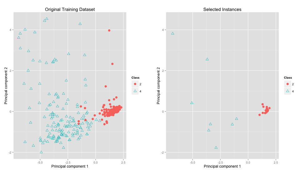
Extras (Wisconsin Breast Cancer)
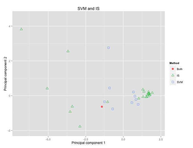
Extras (Ionosphere)
